Gavin R. Putland,  BE PhD

Sunday, December 08, 2013

(Comment)

A self-contained derivation of Kepler's laws from Newton's laws

Kepler's laws of planetary motion, stated with a generality that covers comets as well as planets, are as follows:

1. The orbit of the planet is a conic (ellipse, parabola, or hyperbola) with the sun at one focus.
2. The radius vector — that is, the line segment connecting the sun to the planet — sweeps equal areas in equal times.
3. If the orbit is closed (i.e. elliptical, not parabolic or hyperbolic), the square of the orbital period is proportional to the cube of the semimajor axis of the orbit.

Kepler's laws can be derived from Newton's laws of gravity and motion, subject to the following approximations:

(a) The sun and the planets are so small, by comparison with the distances between them, that they may be regarded as point-masses (i.e. particles).

(b) The gravitational influences of the planets on each other are negligible by comparison with the gravitational influence of the sun on each planet. (This assumption fails spectacularly for a comet or asteroid that has a close encounter with a planet; such cases are not covered by Kepler's laws.)

(c) The mass of the sun is so much larger than those of the planets that the sun can be considered immovable.

The following derivation requires some familiarity with calculus and vectors in the plane, but little else.

Contents

1.  Choosing the coordinates
2.  Velocity and acceleration in polar coordinates
3.  Equations of motion
4.  Kepler's Second Law
5.  The equation of the orbit
6.  Closed orbits, open orbits, forbidden branches
7.  Kepler's First Law
8.  Kepler's Third Law

Appendix: Foci of an elliptical orbit
P.S. (22 May 2018): Solving the DE

1.  Choosing the coordinates

Because the sun is assumed to be stationary, let's choose a coordinate system with the sun at the origin \(O\). Let the planet be at the point \(R\), whose position vector is \({\bf r}\) (the “radius vector”). Hence its velocity is \(\dot{\bf r}\), where the dot denotes differentiation w.r.t. time \(t\). At any time, by Newton's laws, the acceleration of the planet due to gravity is in the direction of \(-{\bf r}\), which is in the plane of \(O\) and \(\dot{\bf r}\), so that \(\dot{\bf r}\) and \({\bf r}\) will not subsequently move out of that plane. Let's choose the coordinate axes to make that plane the \((x,y)\) plane, and let \((x,y)\) be the rectangular coordinates of \(R\).

We are also free to choose the direction of the \(x\) axis; we'll do that later.

The position of \(R\) can also be specified in terms of the polar coordinates \((r,\theta)\), where \(r\) is the (positive) distance from the origin and \(\theta\) is the angle measured anticlockwise from the \(x\) axis, so that \begin{align} x &= r \cos \theta \label{exr}\\ y &= r \sin \theta \label{eyr} \end{align} and \begin{equation}\label{erxy} r = \sqrt{x^2 + y^2}~. \end{equation} Let \({\bf i}, {\bf j}, {\bf e}_r\,, {\bf e}_\theta\) be the unit vectors in the directions of \(x, y, r, \theta,\) respectively, as shown in Fig.1.

Fig.1: Unit vectors (black) for rectangular and polar coordinates.

2.  Velocity and acceleration in polar coordinates

From Fig.1 we see that \begin{equation}\begin{split} {\bf e}_r &= {\bf i} \cos \theta + {\bf j} \sin \theta\\ {\bf e}_\theta &= -{\bf i} \sin \theta + {\bf j} \cos \theta\,. \end{split}\end{equation} Differentiating w.r.t. time using the chain rule, we find that \begin{equation} \begin{split} \dot{\bf e}_r &= \dot{\theta}\,{\bf e}_\theta\\ \dot{\bf e}_\theta &= -\dot{\theta}\,{\bf e}_r\,. \end{split} \label{eunitdot} \end{equation}

In polar coordinates, the position vector of the planet is \begin{equation} {\bf r} = r\,{\bf e}_r\,. \end{equation} Differentiating w.r.t. time, using the product rule and Eqs.\(\,(\ref{eunitdot})\), we obtain \begin{equation} \dot{\bf r} = \dot{r}\,{\bf e}_r + r\dot{\theta}\,{\bf e}_\theta\,, \end{equation} where the first term on the right is the radial velocity and the second is the tangential velocity, while \(\dot\theta\) is called the angular velocity. Differentiating again, we find \begin{align} \ddot{\bf r} &= \ddot{r}\,{\bf e}_r + \dot{r}\dot{\theta}\,{\bf e}_\theta + \dot{r}\dot{\theta}\,{\bf e}_\theta + r\ddot{\theta}\,{\bf e}_\theta - r\dot{\theta}^2{\bf e}_r \label{eaccel}\\ &= (\ddot{r} - r\dot{\theta}^2)\,{\bf e}_r + (r\ddot{\theta} + 2\dot{r}\dot{\theta})\,{\bf e}_\theta\,. \label{eacomp} \end{align}

[Digression: In \((\ref{eaccel})\), the first \(\dot{r}\dot{\theta}\,{\bf e}_\theta\) term comes from the changing direction of the radial velocity, while the second comes from the changing magnitude of the tangential velocity, due to the changing radius. The sum of these terms, known as the Coriolis acceleration, is the reason why it's hard to walk straight in a radial direction on a rotating platform, such as a playground carousel (Fig.2). The term \(r\ddot{\theta}\,{\bf e}_\theta\) comes from the changing magnitude of the tangential velocity, due to the changing angular velocity. The term \(-r\dot{\theta}^2{\bf e}_r\) is the centripetal acceleration and is due to the changing direction of the tangential velocity. Hence, in \((\ref{eacomp})\), \(-r\dot{\theta}^2\) is the centripetal term and \(2\dot{r}\dot{\theta}\) is the Coriolis term.]

3.  Equations of motion

Let \({\bf F}\) be the force of gravity acting on the planet. By Newton's second law of motion, \begin{equation} {\bf F} = m\,\ddot{\bf r}\,, \end{equation} where \(m\) is the mass of the planet. And by Newton's law of gravity, \begin{equation}\label{egrav} {\bf F} = \frac{-GMm}{r^2}\,{\bf e}_r\,, \end{equation} where \(G\) is the gravitational constant (about \(6.674\times 10^{-11}\,{\rm N}{\rm m}^2{\rm kg}^{-2}\)), and \(M\) is the mass of the sun (about \(1.9885\times 10^{30}\,{\rm kg}\)). When we equate the two expressions for \({\bf F}\), the planetary mass \(m\) cancels out, and we get \begin{equation}\label{emot} \ddot{\bf r} = \frac{-GM}{r^2}\,{\bf e}_r\,. \end{equation} Thus the acceleration due to gravity is independent of the mass of the planet (subject to the initial assumption that the mass of the planet is very small compared with that of the sun — which is true for, e.g., an earth-sized planet or a golf-ball-sized “planet”).

If we substitute \((\ref{emot})\) into \((\ref{eacomp})\), equating the coefficients of \({\bf e}_r\) (the radial components) gives \begin{equation}\label{ear} \ddot{r} - r\dot{\theta}^2 = \frac{-GM}{r^2}\,, \end{equation} and equating the coefficients of \({\bf e}_\theta\) (the tangential components) gives \begin{equation}\label{eath} r\ddot{\theta} + 2\dot{r}\dot{\theta} = 0\,. \end{equation}

4.  Kepler's Second Law

In the infinitesimal time \(dt\), the infinitesimal area \(dA\) swept by the radius vector is the area of a triangle whose base length is \(r\) and whose perpendicular height is \(r\,d\theta=r\dot{\theta}\,dt\). So the area (half the base times the perpendicular height) is \[ dA = \tfrac{1}{2}r^2\dot{\theta}\,dt\,. \] Hence the rate at which area is swept, which is called the areal velocity, and which we shall denote by \(K\), is \begin{equation}\label{eK} K = \tfrac{1}{2}r^2\dot{\theta}\,. \end{equation} Differentiating w.r.t. time gives \begin{align} \dot{K} &= \tfrac{1}{2}\big(r^2\ddot{\theta}+2r\dot{r}\dot{\theta}\big)\\ &= \tfrac{r}{2}\big(r\ddot{\theta}+2\dot{r}\dot{\theta}\big)\\ &= 0\,, \end{align} where the last equality follows from \((\ref{eath})\). Therefore \(K\) is constant — that is, area is swept at a constant rate, so equal areas are swept in equal times.

[Digression: From \((\ref{eK})\), the reader may notice that \(2mK\) is the angular momentum of the planet about the \(z\) axis. Thus the constancy of \(K\) (Kepler's second law) expresses conservation of angular momentum. Eq.\(\,(\ref{ear})\) depends on the fact that the force of gravity is proportional to the inverse square of the radius. But Kepler's second law comes from \((\ref{eath})\), which doesn't depend on the inverse-square law. It doesn't even depend on the fact that the magnitude of the force is independent of \(\theta\), or that the force is attractive rather than repulsive. It depends only on the fact that the force has no component in the \(\theta\) direction. But Kepler's first and third laws do depend on the inverse-square law, as we shall see.]

5.  The equation of the orbit

For reasons which will soon become apparent, let's define \begin{equation}\label{esr} s = 1/r\,, \end{equation} i.e. \begin{equation}\label{ers} r = s^{-1}, \end{equation} so that \((\ref{eK})\) becomes \begin{equation}\label{ethdot} \dot{\theta} = 2Ks^2\,. \end{equation} Let a prime (\('\)) denote differentiation w.r.t. \(\theta\). Then, from \((\ref{ers})\) and the chain rule, we obtain \begin{equation}\label{erprime} r' = -s^{-2}s' \end{equation} and \begin{equation} \dot{r} = r'\dot{\theta}\,, \end{equation} and the latter may be differentiated again to obtain \begin{equation}\label{erddot} \ddot{r} = \big( r'\dot{\theta}\big)'\,\dot{\theta}\,. \end{equation} Substituting \((\ref{ethdot})\) and \((\ref{erprime})\) into \((\ref{erddot})\) and simplifying, we find \begin{equation}\label{erddots} \ddot{r} = -4K^2s^2s''. \end{equation} Then, substituting \((\ref{ers})\), \((\ref{ethdot})\), and \((\ref{erddots})\) into \((\ref{ear})\) and simplifying, we obtain the differential equation \begin{equation}\label{esde} s'' + s = \frac{GM}{4K^2}\,, \end{equation} whose general solution (easily verified by substitution) is \begin{equation}\label{esgen} s = \frac{GM}{4K^2}\big(1 + e\cos[\theta+\phi]\big)\,, \end{equation} where \(e\) and \(\phi\) are constants.

Let's choose the constants so that \(e\) is non-negative (this is possible because adding \(\pi\) to \(\phi\) is equivalent to changing the sign of \(e\)). Remember that we are also free to choose the direction of the \(x\) axis. Let's choose it so that \(\phi\!=\!0\). Then, invoking \((\ref{esr})\), we have \begin{equation}\label{erth} \frac{1}{r} = \frac{GM}{4K^2}\big(1 + e\cos\theta\big)\,. \end{equation} Because \(e\) is non-negative and \(GM\big/(4K^2)\) is positive, the maximum value of \(1/r\), hence the minimum value of \(r\), occurs where \(\theta\!=\!0\). That minimum value of \(r\), which is the perihelion distance of the planet, is found to be \begin{equation}\label{ep} p = \frac{4K^2}{GM(1+e)}\,. \end{equation} Hence \((\ref{erth})\), which is the equation of the orbit in polar coordinates, can be rewritten in terms of \(p\) as \begin{equation}\label{erpth} \frac{1}{r} = \frac{1+e\cos\theta}{p(1+e)}\,. \end{equation}

6.  Closed orbits, open orbits, forbidden branches

Eq.\(\,(\ref{erpth})\) indicates that \(1/r\) is a smooth periodic function of \(\theta\), with period \(2\pi\).

If \(0\!\leq\!e\!\lt\!1\), then \(1/r\) is positive for all \(\theta\), so that \(r\) remains positive and finite for all \(\theta\). Thus the orbit is a closed curve.

If \(e\!=\!1\), then as \(\theta\) approaches \(\pm\pi\), the reciprocal of \(r\) approaches zero, so that \(r\) increases without limit (“approaches infinity”). For \(\theta\!=\!\pm\pi\), the value of \(r\) is undefined and the orbit is open.

If \(e\!\gt\!1\), then \(1/r\!\rightarrow\!0\) as \(\theta\!\rightarrow\!\pm\arccos(-1/e)\). For \(\theta\!=\!\pm\arccos(-1/e)\), the value of \(r\) is undefined and the orbit is open. For the range of \(\theta\) for which \((\ref{erpth})\) gives a negative value of \(r\), the equation describes a forbidden branch of the orbit, because \(r\) is defined as positive.

[Digression: If \(r\) were negative, the unit vector \({\bf e}_r\) would point towards the origin, in which case our assumption that the force of gravity is in the direction of \(-{\bf e}_r\) [Eq.(\(\ref{egrav})\)] would amount to an assumption that the force is away from the origin. Thus the forbidden branch would be a permitted orbit if the force of gravity were repulsive rather than attractive.]

7.  Kepler's First Law

By (\(\ref{erpth})\), \begin{align} p(1+e) &= r(1+e\cos\theta) \nonumber\\ &= r + e(r\cos\theta) \nonumber\\ &= r + ex\,, \label{eprx} \end{align} so that \begin{equation}\label{econic} r = e\left[p\big(1+\tfrac{1}{e}\big) - x\right]. \end{equation} If \((x,y)\) and \((r,\theta)\) are the rectangular and polar coordinates of the point \(R\), then \(r\) is the distance of \(R\) from the origin \(O\), and the expression in square brackets is the perpendicular distance of \(R\) from the line \(\mathcal D\) whose constant \(x\) coordinate is \begin{equation}\label{exd} x_D = p\big(1+\tfrac{1}{e}\big) \end{equation} (see Fig.3). Thus Eq.(\(\ref{econic})\) says that the distance of \(R\) from the point \(O\) is \(e\) times the distance of \(R\) from the line \(\mathcal D\,\); that is, \(R\) lies on a conic with focus \(O\), eccentricity \(e\), and directrix \(\mathcal D\).

The conclusion that the focus is at the origin applies for all values of \(e\). If \(e\!\gt\!1\), the conic is a hyperbola. If \(e\!=\!1\), the conic is a parabola (open in the \(-x\) direction). If \(0\!\lt\!e\!\lt\!1\), the conic is an ellipse (closed) as in Fig.3. If \(e\!=\!0\), we can't use (\(\ref{econic})\), but (\(\ref{eprx})\) reduces to \(r\!=\!p\), which describes a circle (a special case of an ellipse).

The focus-directrix formulation has the advantage that it covers all values of \(e\). But if \(e\!\lt\!1\), a different formulation makes it more obvious that the orbit is an ellipse — as we shall see.

8.  Kepler's Third Law

In \((\ref{erpth})\), putting \(\theta\!=\!0\) gives \[r=p\,,\] and putting \(\theta\!=\!\pi\) gives \[r=\tfrac{p(1+e)}{1-e}\,.\] If \(e\!\lt\!1\), the semiaxis of the orbit in the \(x\) direction, denoted by \(a\), is half the sum of the two values of \(r\,\); that is, \[ a = \tfrac{1}{2}\Big(p + \tfrac{p(1+e)}{1-e}\Big) = \tfrac{p}{1-e}\,, \] whence \begin{equation}\label{epa} p = a(1\!-\!e) \end{equation} (as indicated in Fig.3). Substituting from \((\ref{epa})\), we can rewrite \((\ref{ep})\) and \((\ref{eprx})\) as \begin{equation}\label{eKsq} K^2 = \tfrac{1}{4}{GMa(1-e^2)} \end{equation} and \begin{equation}\label{erax} r = a(1\!-\!e^2) - ex\,. \end{equation} Substituting \((\ref{erxy})\) into \((\ref{erax})\), squaring both sides, expanding, and grouping terms, we get \begin{equation}\label{exyexp} (1\!-\!e^2)\,x^2 + 2a(1\!-\!e^2)\,ex + y^2 = a^2(1\!-\!e^2)^2. \end{equation} Dividing through by \(a^2(1\!-\!e^2)\) gives \[ \left(\tfrac{x}{a}\right)^2 + 2\tfrac{x}{a}e + \left(\frac{y}{a\sqrt{1\!-\!e^2}}\right)^{\!2\!} = 1-e^2. \] Adding \(e^2\) to both sides, thereby completing the square on the first two terms, we obtain the equation of the orbit in rectangular coordinates: \begin{equation}\label{exyell} \left(\frac{x+ae}{a}\right)^{\!2\!}+\left(\frac{y}{a\sqrt{1\!-\!e^2}}\right)^{\!2\!} = 1\,. \end{equation}

By way of comparison, if the equation of the orbit were \[ (x+ae)^2 + y^2 = 1\,, \] the orbit would obviously be a circle of radius \(1\), centered on the point \((-ae,0)\), and the enclosed area would be \(\pi\). The denominators in \((\ref{exyell})\) do not shift the centre (indicated by \(C\) in Fig.3), but stretch the circle by the factor \(a\) in the \(x\) direction and the smaller factor \(a\sqrt{1\!-\!e^2}\) in the \(y\) direction, so that the area is increased by the factor \(a^2\sqrt{1\!-\!e^2}\).

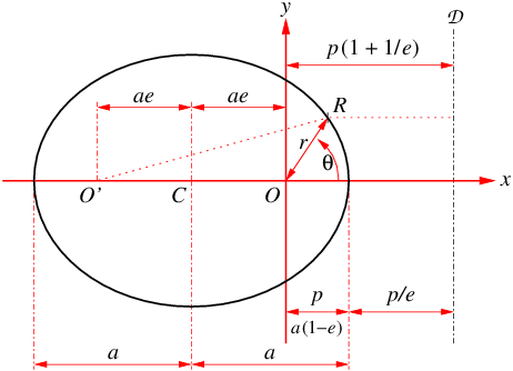
Fig.3: Elliptical orbit with perihelion distance \(p\), focus \(O\), directrix \({\mathcal D}\), eccentricity \(e\), and semimajor axis \(a\).

So the circle becomes an ellipse with semimajor axis \(a\) in the \(x\) direction (see Fig.3), and semiminor axis \(a\sqrt{1\!-\!e^2}\) in the \(y\) direction; and the enclosed area becomes \begin{equation}\label{eA} A = \pi a^2 \sqrt{1\!-\!e^2}\,. \end{equation}

Because \(K\) is constant, the orbital period is \(T=A/K\), so that \begin{equation}\label{eTsq} T^2=A^2\big/K^2. \end{equation} Substituting \((\ref{eKsq})\) and \((\ref{eA})\) into \((\ref{eTsq})\) gives \begin{equation}\label{eK3} T^2 = \frac{4\pi^2}{GM}\,a^3\,, \end{equation} showing that \(T^2\) is proportional to \(a^3\).

Appendix: Foci of an elliptical orbit

In Fig.3, the points \(O\) and \(O'\) are on opposite sides of the centre \(C\), and equidistant from it. From the symmetry of the figure described by \((\ref{exyell})\), we conclude that \(O'\) is a focus of the ellipse. Hence, from the dimensions in Fig.3, we obtain another definition of \(e\): the eccentricity of an ellipse is the ratio of the interfocal distance to the major axis.

We can confirm that \(O\) and \(O'\) are foci by another method. If \(R\) is on the \(x\) axis, the dimensions in Fig.3 indicate that the sum of the distances \(OR\) and \(O'R\) is \(2a\). Let's find the equation of the curve that satisfies the same “sum of the distances” constraint for all points on the curve: \begin{align} 2a &= \text{\(O\)\(R\)} + \text{\(O'\)\(R\)} \label{e2foci}\\ &= \sqrt{x^2 + y^2} + \sqrt{(x+2ae)^2 + y^2}\,. \nonumber \end{align} Transposing \(\sqrt{x^2 + y^2}\) to the left-hand side, then squaring both sides, expanding completely, and simplifying, we get \[ \sqrt{x^2 + y^2} = a(1\!-\!e^2) - ex\,. \] Squaring both sides again, we get \((\ref{exyexp})\), which leads to \((\ref{exyell})\), which is the previously determined equation of the orbit in rectangular coordinates.

Eq.\(\,(\ref{e2foci})\) is the two-focus definition of an ellipse. As it yields the same orbit as the focus-directrix definition \((\ref{econic})\), it confirms that \(O'\) is the other focus.

The two-focus definition explains why you can draw an ellipse with two pins (one on each focus) and a loop of string; from Fig.3, we see that the perimeter of the loop is \(2a(1\!+\!e)\). It also explains the reflective property of an elliptical boundary: waves radiating from one focus and reflecting off the boundary converge on the other focus, because the number of wavelengths in the path from one focus to the boundary and back to the other focus is the same for all points on the boundary.

[Last modified 29 May 2016.]

P.S. (22 May 2018): Solving the DE

I have been asked whether you can deduce \((\ref{esgen})\) from \((\ref{esde})\), rather than simply verifying that \((\ref{esgen})\) satisfies \((\ref{esde})\), if you only know about first-order differential equations (DEs).

Well, that's not the easiest approach, but... Yes, you can, provided that you know one extra trick. Remembering that the prime denotes differentiation w.r.t. \(\theta\), we have \begin{align*} \frac{d}{ds}\left(\tfrac{1}{2}(s')^2\right) &= s'\frac{ds'}{ds} = \frac{ds'}{ds}s' = \frac{ds'}{ds}\frac{ds}{d\theta} = \frac{ds'}{d\theta}\\[2ex] &= s''. \end{align*} Substituting this into \((\ref{esde})\) gives \[ \frac{d}{ds}\left(\tfrac{1}{2}(s')^2\right) = \frac{GM}{4K^2} - s\,, \] hence \[ \tfrac{1}{2}(s')^2 = C + \tfrac{GM}{4K^2} s - \tfrac{1}{2}s^2\, \] where \(C\) is the arbitrary constant of integration. Solving for \(s'\) (i.e., \(ds/d\theta\)), we get \[ \frac{ds}{d\theta} = \pm\sqrt{2C + \tfrac{GM}{2K^2}s - s^2}\,, \] which is separable: \begin{align*} d\theta &= \frac{ds}{\pm\sqrt{2C - \big(s^2-\tfrac{GM}{2K^2}s\big)}}\\[1ex] &= \frac{ds}{\pm\sqrt{2C + \big(\tfrac{GM}{4K^2}\big)^2 - \big(s - \tfrac{GM}{4K^2}\big)^2}} \end{align*} (“completing the square”).  Now  \(2C + \big(\tfrac{GM}{4K^2}\big)^2\) is just an arbitrary constant (because \(C\) is); so let us rename it \(E^2\). And let us define the new variable \begin{equation}\label{eus} u = s - \tfrac{GM}{4K^2}\,. \end{equation} Then we have \[ d\theta = \frac{du}{\pm\sqrt{E^2-u^2}}\,. \] With the further substitution \begin{equation}\label{eups} u = E\cos\psi\,, \end{equation} we get \[ d\theta = \frac{-E\sin\psi\,d\psi}{\pm E\sin\psi} = \mp d\psi\,. \] Integrating gives \[ \theta + \phi = \mp\psi\,, \] where \(\phi\) is the arbitrary constant of integration. Hence \begin{align*} E\cos(\theta+\phi) &= E\cos(\mp\psi) &&\\ &= E\cos\psi &&\\ &= u && \text{by \((\ref{eups})\).} \end{align*} Substituting this into \((\ref{eus})\) and rearranging, we get \[ s = \tfrac{GM}{4K^2} + E\cos(\theta+\phi)\,. \] Then, since \(E\) is an arbitrary constant, we can write it as \(\tfrac{GM}{4K^2}e\), where \(e\) is another arbitrary constant. That gives \((\ref{esgen})\).

All of which reminds us that it is easier to verify that \((\ref{esgen})\) satisfies \((\ref{esde})\).

---

Tweet

Return to Contents

comments powered by Disqus